Double Pendulum Example

A double pendulum is a dynamic system which has chaotic mostion for many initial conditions.

The derivation of the derivative function for this example is taken from https://myphysicslab.com/pendulum/double-pendulum-en.html

When the system is defined as a series of first-order differential equations the state vector is

\[ \begin{align}\begin{aligned}\begin{split} X = \begin{bmatrix} \theta_1 \\ \theta_2 \\ \omega_1 \\ \omega_2 \end{bmatrix}\end{split}\\and the derivative of the system is\end{aligned}\end{align} \]

\[\begin{split}\dot{X} = \begin{bmatrix} \dot{\theta_1} \\ \dot{\theta_2} \\ \dot{\omega_1} \\ \dot{\omega_2} \end{bmatrix} = \begin{bmatrix} \omega_1 \\ \omega_2 \\ \frac{-g (2 m_1 + m_2) \sin{\theta_1} - m_2 g \sin(\theta_1 - 2 \theta_2) - 2 \sin(\theta_1 - \theta_2) m_2 (\omega_2^2 L_2 + \omega_1^2 L_1 \cos(\theta_1 - \theta_2))}{L_1 (2 m_1 + m_2 - m_2 \cos(2 \theta_1 - 2 \theta_2))} \\ \frac{2 \sin(\theta_1 - \theta_2)(\omega_1^2 L_1 (m_1 + m_2) + g (m_1 + m_2) \cos{\theta_1} + \omega_2^2 L_2 m_2 \cos(\theta_1 - \theta_2))}{L_2 (2 m_1 + m_2 - m_2 \cos(2 \theta_1 - 2 \theta_2))} \end{bmatrix}.\end{split}\]

cd ..

/home/docs/checkouts/readthedocs.org/user_builds/ode-solver/checkouts/master

import numpy as np
import ode
import matplotlib.pyplot as plt
from matplotlib.animation import FuncAnimation
from IPython.display import HTML

def doublependulum(t,X):
    th1, th2, om1, om2 = X
    g = 9.81
    m1 = 1
    m2 = 1
    l1 = 1
    l2 = 1
    k1 = -g * ((2 * m1) + m2) * np.sin(th1)
    k2 = m2 * g * np.sin(th1 - (2 * th2))
    k3 = 2 * np.sin(th1 - th2) * m2
    k4 = ((om2**2) * l2) + ((om1**2) * l1 * np.cos(th1 - th2))
    k5 = m2 * np.cos((2 * th1) - (2 * th2))
    k6 = 2 * np.sin(th1 - th2)
    k7 = ((om1**2) * l1 * (m1 + m2))
    k8 = g * (m1 + m2) * np.cos(th1)
    k9 = (om2**2) * l2 * m2 * np.cos(th1 - th2)
    dX = np.array([
        om1,
        om2,
        (k1 - k2 - (k3 * k4)) / (l1 * ((2 * m1) + m2 - k5)),
        (k6 * (k7 + k8 + k9)) / (l2 * ((2 * m1) + m2 - k5))
    ])
    return dX

def angles2xy(th1, th2, om1, om2):
    l1 = 1
    l2 = 1
    x1 = l1 * np.sin(th1)
    y1 = -l1 * np.cos(th1)
    x2 = x1 + (l2 * np.sin(th2))
    y2 = y1 - (l2 * np.cos(th2))
    return x1, y1, x2, y2


et, ex = ode.euler(doublependulum, [np.pi/2,np.pi,0,0], [0,5], .025)
th1, th2, om1, om2 = ex
ex1, ey1, ex2, ey2 = zip(*[angles2xy(*xi) for xi in zip(th1, th2, om1, om2)])

bet, bex = ode.backwardeuler(doublependulum, [np.pi/2,np.pi,0,0], [0,5], .025)
bex1, bey1, bex2, bey2 = zip(*[angles2xy(*xi) for xi in zip(*bex)])

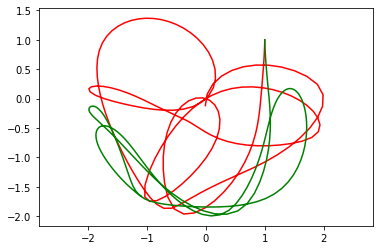
fig, ax = plt.subplots()
ax.plot(ex2, ey2, 'r', bex2, bey2, 'g')
ax.set_aspect('equal', 'datalim')
plt.show()

#plt.rcParams['figure.dpi'] = 120
fig, ax = plt.subplots()
ax.axis([-2, 2, -2, 2])
ax.set_aspect('equal')
trace_euler, = plt.plot([], [], 'r', animated=True)
pend_euler, = plt.plot([], [], 'ro-', animated=True)
trace_backeuler, = plt.plot([], [], 'g', animated=True)
pend_backeuler, = plt.plot([], [], 'go-', animated=True)
anim_ex2 = []
anim_ey2 = []
anim_bex2 = []
anim_bey2 = []

def update(frame):
    anim_ex2.append(ex2[frame])
    anim_ey2.append(ey2[frame])
    pend_euler_x = [0, ex1[frame], ex2[frame]]
    pend_euler_y = [0, ey1[frame], ey2[frame]]
    anim_bex2.append(bex2[frame])
    anim_bey2.append(bey2[frame])
    pend_backeuler_x = [0, bex1[frame], bex2[frame]]
    pend_backeuler_y = [0, bey1[frame], bey2[frame]]
    trace_euler.set_data(anim_ex2, anim_ey2)
    pend_euler.set_data(pend_euler_x, pend_euler_y)
    trace_backeuler.set_data(anim_bex2, anim_bey2)
    pend_backeuler.set_data(pend_backeuler_x, pend_backeuler_y)
    return trace_euler, pend_euler, trace_backeuler, pend_backeuler

%matplotlib inline
ani = FuncAnimation(fig, update, frames=range(len(et)), blit=True)

HTML_ani = HTML(ani.to_jshtml())
#HTML_ani = HTML(ani.to_html5_video())
#ani.save('DoublePendulumExample.gif', writer='imagemagick', fps=60)
HTML_ani

Once Loop Reflect